 Spectryse
Media and playback
- Import media. MP4, MKV, MOV, WAV, FLAC and MP3, plus other common audio and video formats such as WebM, AAC and OGG.
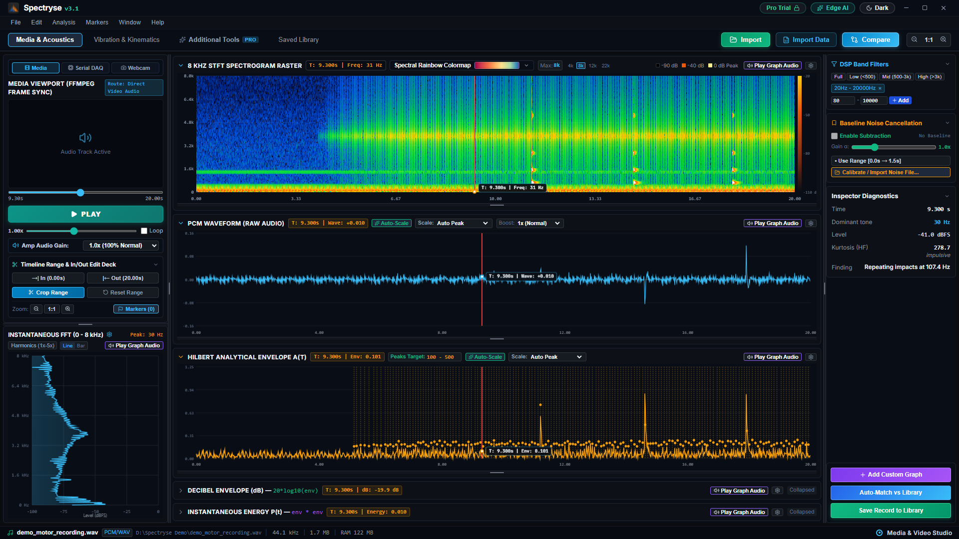
- Video beside the graphs. Frame-accurate video preview, so you can see what the machine was doing at the moment of a sound.
- Synchronised views. Spectrogram, waveform, Hilbert envelope and the instantaneous FFT at the playhead, all on one timeline.
- Read the values. Hover the spectrogram to read the frequency and level. Switch between logarithmic and linear frequency scales, and choose a colour map.
- Playback control. Speeds from 0.25x to 2.0x, loop, and the space bar to play or pause. Zoom with the mouse wheel. Set in and out points to crop a clip.
- Markers. Bookmark events on the timeline with notes, and export them to CSV.
Filters and signal tools
- Filter presets. Full, low, mid and high bands, or a custom band, using 4-pole Butterworth filters.
- Hilbert envelope. The instantaneous amplitude of the signal. Spikes show clicks, knocks and friction bursts.
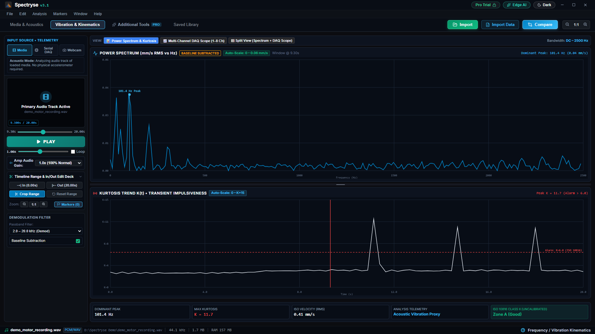
- Kurtosis trend. A sliding kurtosis curve across the clip, with an alarm threshold, to show how impulsive the signal is.
- Transient detection. Finds sharp impacts automatically and lists them by time.
- Custom graphs. Add your own equation graphs over the signal, for example the envelope squared or the envelope in decibels, and save the layout.
Library matching
- Save to Library. Store a recording as a reference signature for future comparisons.
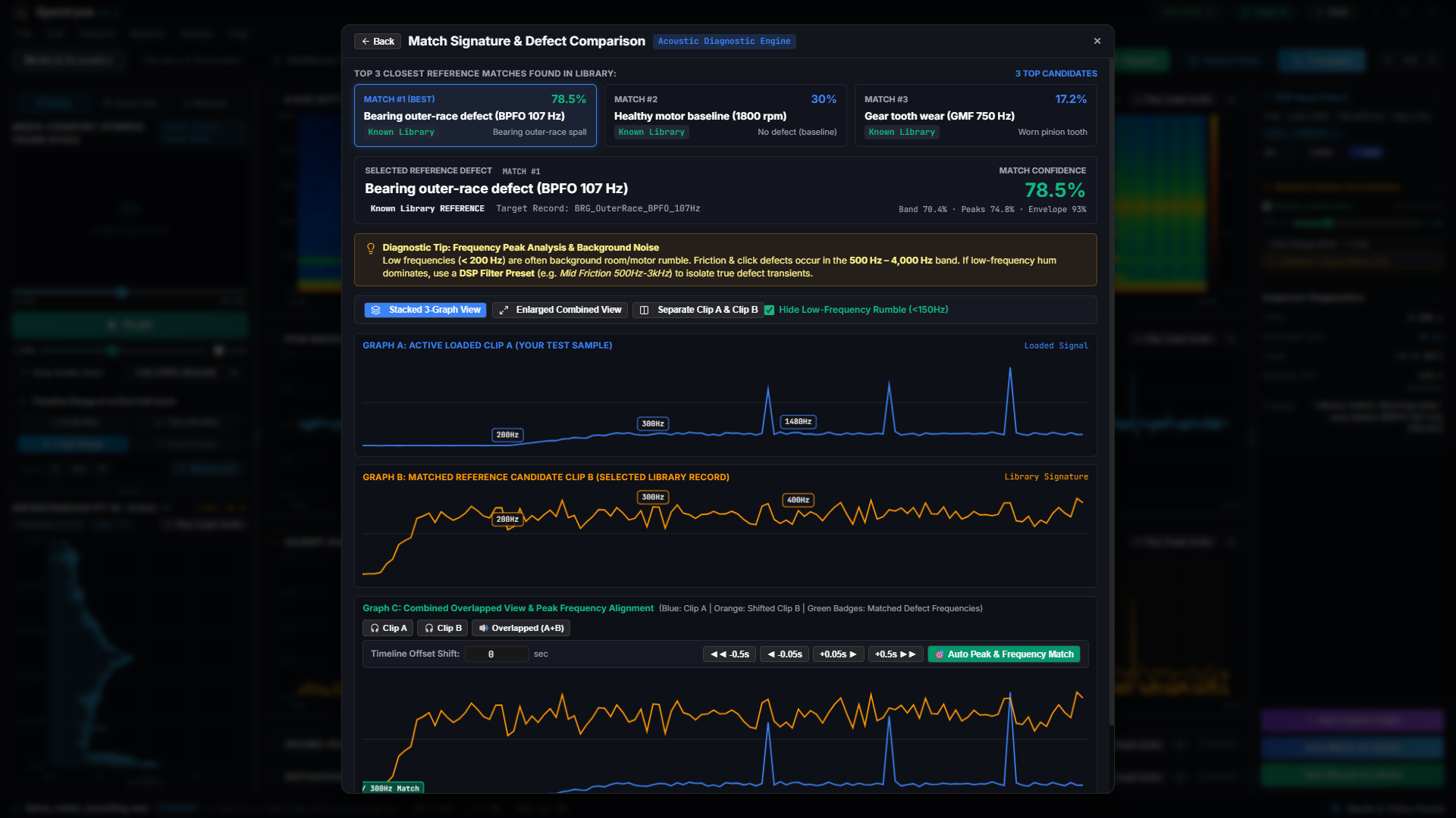
- Match from Library. Compares the sound of the active recording with every reference signature in your library and shows the three closest matches. The score combines three comparisons: the 1/6-octave band spectrum, the prominent tones, and the envelope spectrum that shows how often impacts repeat. 100% means the same features; each match shows how the three parts scored. Each match also has the profile name in plain words and a suggested action.
- Level-independent. Scores compare the shape of the sound, not its loudness or length, so recordings made at different distances or with different gain compare fairly.
- Compare views. Stacked graphs, an enlarged combined view, or the two clips separately. Matching peak frequencies are marked. An option hides rumble below 150 Hz so the useful peaks stay clear.
- Root cause notes. A 5-Whys section under the comparison keeps root cause statements and corrective actions with the result.
- A/B alignment. Overlay a reference recording and line up the peaks automatically by cross-correlation, or shift the time by hand in milliseconds.
Baseline subtraction
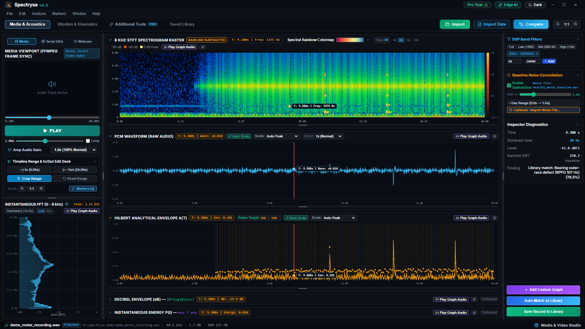
- Baseline subtraction. Set a known-good recording as the baseline, or pick one from the library. Turn on subtraction and its average spectrum is removed from the spectrogram, the live spectrum and the vibration spectrum. A gain slider sets how much is removed. The waveform and the audio are left as recorded.
- Severity stays honest. The ISO severity reading always uses the full signal, even while subtraction is on.
Vibration
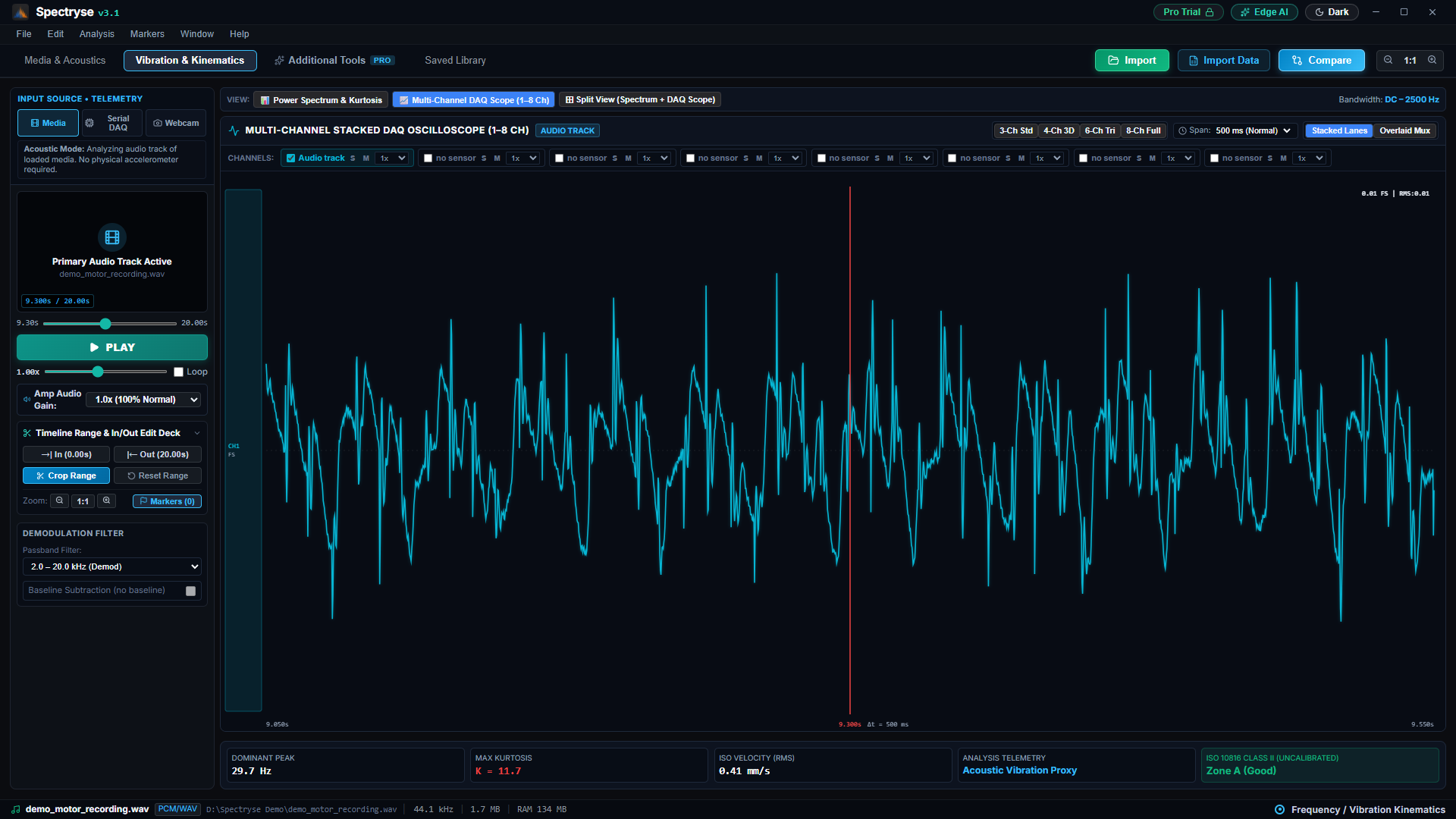
- Velocity spectrum. Vibration velocity in mm/s RMS against frequency, with the dominant peak marked.
- ISO 10816 and ISO 20816 severity. Overall velocity graded into zone A (good), B (acceptable), C (alert) or D (danger), with a pass or fail verdict.
- Bearing fault frequencies. BPFO, BPFI, BSF and FTF from the bearing geometry and shaft speed.
- Gearbox frequencies. Gear mesh frequency and its 2x and 3x harmonics, hunting tooth frequency, and pinion and gear sidebands.
- Envelope spectrum. Band-pass a resonance, take its envelope and look at the low-frequency spectrum to find repeating bearing impacts.
- Scope view. The recording as a scope trace, with gain and time spans from 50 ms to 5 s. Extra lanes stay empty until a sensor source supplies more channels; nothing is made up from the audio.
- No accelerometer? The vibration tools also work on the audio of an imported recording.
Advanced analysis
- Fast kurtogram. Spectral kurtosis across a tree of frequency bands finds the band where impacts dominate. One click applies that band as a filter.
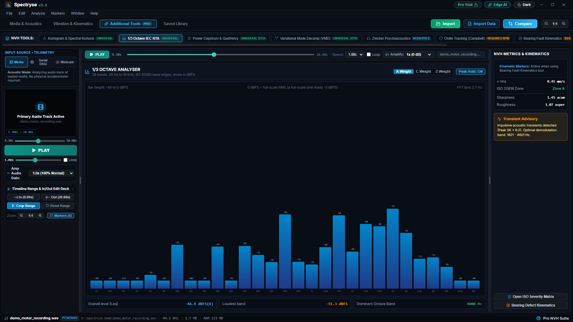
- 1/3-octave bands. 29 bands from 25 Hz to 16 kHz with A, C or Z weighting, in dBFS (a full-scale sine reads −3 dBFS).
- Order tracking. Orders against speed in a Campbell diagram, for run-ups and coast-downs. This needs a tachometer signal; a plain recording has no speed reference.
- Power cepstrum. Finds families of evenly spaced harmonics and sidebands.
- Psychoacoustics. Zwicker loudness in sones and sharpness in acum (a 1 kHz tone reads about 1 acum). Without a calibrated microphone, treat loudness as a guide.
- Coherence. Magnitude-squared coherence and phase lag between two signals, to trace a path from source to sensor.
Live inputs
- Audio input. Analyse a microphone or other audio input live.
- USB serial. Connect a serial data logger, such as an accelerometer board or an optical tachometer, and set the port, baud rate and sample rate.
- Live comparison. Compare the live signal with a library reference, inside a tolerance band in dB. Freeze and capture an anomaly to the library.
- Rewind. Scrub back through the last 30 seconds of the live signal and send a slice to the analysis workspaces.
Data interchange and reports
| Format | Import | Export |
|---|---|---|
| Universal File Format, dataset 58 (.unv, .uff) | Yes | Yes |
| Engineering CSV and TSV time series (headers, units and sample rate detected) | Yes | Yes |
| Reports: results, timestamps and suggested actions (CSV or Excel .xlsx) | No | Yes |
| Markers: Audacity label track (.txt), Sonic Visualiser (.xml) | No | Yes |
| MATLAB or Python data (.json) | No | Yes |
Engineering CSV export can include the raw signal, the filtered signal, the envelope and the kurtosis series.
Assistant
A built-in assistant answers questions about the active recording: the main peaks and their harmonics, the ISO severity zone, bearing fault frequencies and transient impacts. It runs on your computer.
If you prefer, you can point it at a local model server, such as Ollama or LM Studio, or at a cloud provider you choose. A cloud provider receives your questions and a summary of the analysis, under that provider's own terms.